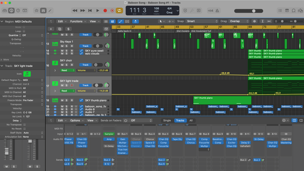
Here’s something playful for you — Baboon Song, a track I composed using temporal networks:
I took the Baboons’ interactions dataset from SocioPatterns, turned some baboon interaction timelines into MIDI files, chopped the files into bits, and constructed loops by feeding them into various synths in Ableton Live. I built the skeleton of the song in Ableton, added more instruments, and mixed the track in Logic Pro X (a tool I know better than Live).
The repeating rhythmic patterns are interaction timelines corresponding to a day in some baboon’s life — the pattern that starts the song is between two baboons, and the bell-like pattern that enters next is a whole temporal ego-net of another baboon. There are whispers of other ego-nets in the L and R channels… On top of the baboon sounds, I added a bit of synth bass, a few rhythmic elements, and some slightly cheesy harmony at the end of the track that I felt just had to be there, because of sunrise over the savannah or something.
Enjoy!!
PS If there is a production nerd among you who wonders — rightly so — what the beautiful, spacious reverb that everything swims in is, it’s just the default preset of Valhalla’s VintageVerb. The best reverb that there is. Rant over.
I recently gave a talk at the Complexity, Aesthetics, and Sonification workshop in Bielefeld, Germany, organized by Thilo Gross, Maximilian Schich, and Cristián Huepe. A really great workshop with lots of different points of view from art to science!
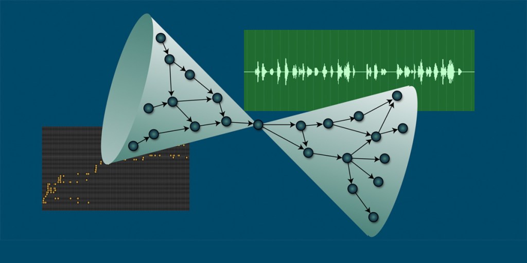
For the talk, I did a bit of exploration in representing temporal networks with sounds. As those who have dabbled with temporal networks know, visualizing them is very difficult, as they live in time instead of space. But so do sounds. Let’s hear what temporal networks sound like, then!
So what was that? That was one month’s worth of data on students’ phone calls from the Copenhagen experiment, compressed into 13 seconds. I took 10 random students and assigned each their own random pitch so that a sound is played every time the student makes a call. I then turned the time series into MIDI which was fed into one of the synthesizers of Apple’s Logic Pro X.
For such a simple and straightforward exercise, there’s a surprising amount of information in the sonification. If you are into temporal networks, you can hear several familiar patterns: there is a daily cycle, weekdays are different from weekends, and there’s also burstiness.
Let’s continue listening to these data. The Copenhagen data set contains metadata on text messages as well, so let’s pick one of the students and listen to their egonets — everyone they call or text will get their own pitch, so that, e.g., one friend is always C (on some octave). Then we’ll feed the calls into a sampler with piano sounds and the texts into another with sampled upright bass.
Quite jazzy, isn’t it? And, again, one can pick up a lot of information here. The daily cycle and the burstiness are still there — and there are even some repeated patterns, parts of temporal motifs. There is also a finding that had escaped my attention earlier — at around the middle of the timeline, there is a cluster of notes being played on the piano, as the student makes a large number of calls in a short period of time. This pattern is, in fact, present in several other students’ timelines at the very same time.
Now let’s have a bit of fun with probing the network with random walkers. I use greedy walkers — a random walker is placed on a node (student), and when the student makes a phone call, the walker moves on to the student being called, and so on. Every newly visited student gets their own pitch that is one semitone higher; when the pitch goes down during the process, this means that the walker is visiting nodes that were already visited. Let’s hear one walk, starting from a random node:
The walker explores a larger subnetwork around the starting point, sometimes backtracking, before escaping off. Now let’s hear another walk:
Quite different, right? This walker has literally become stuck in a neighbourhood of a few students who only keep calling one another and the walker cannot escape. So the social neighbourhoods of these two students are quite different indeed!
Finally, for something entirely different — the sound of criticality. This is simulated (by my student Sara Laurila): what we have is the SIS (Susceptible-Infectious-Susceptible) model on a N=50000 node network, parametrized exactly at criticality — on the boundary between two phases where in one, all activity dies out and in the other, there is persistent activity. (In the model, nodes are S until they are in contact with an I, then they become I and make others I too, until they revert back to being S, to become I again at some point in the future. So this excitement (I) propagates through the network).
In the sonification below, I again use a random sample of sentinel nodes, each assigned their own random pitch. The nodes make a sound whenever they turn I, i.e., whenever the wave of excitation hits them. Here’s what criticality sounds like:
Here’s the same but with drum sounds instead. Sounds like Zappa, but without intention or direction, as a drummer friend of mine remarked.
And finally, criticality from the point of view of one single sentinel node:
Rejoice! There is a new book on temporal networks coming out soon — Temporal Network Theory, edited by Petter Holme & myself. A lot has happened in temporal-network research since our first edited volume (Temporal Networks, 2013); in this new volume, we wanted to focus on the theoretical side of things & invited contributions from many pioneering scientists & groups.
As a teaser trailer, here is a list of the book’s chapters:
A Map of Approaches to Temporal Networks—Petter Holme and Jari Saramäki
Fundamental Structures in Temporal Communication Networks—Sune Lehmann
Weighted, Bipartite, or Directed Stream Graphs for the Modeling of Temporal Networks—Matthieu Latapy, Clémence Magnien, Tiphaine Viard
Modelling Temporal Networks with Markov Chains, Community Structures and Change Points—Tiago P. Peixoto and Martin Rosvall
Visualisation of Structure and Processes on Temporal Networks—Claudio D. G. Linhares, Jean R. Ponciano, Jose Gustavo S. Paiva, Bruno A. N. Travençolo, Luis E. C. Rocha
Weighted Temporal Event Graphs—Jari Saramäki, Mikko Kivelä, Márton Karsai
Exploring Concurrency and Reachability in the Presence of High Temporal Resolution—Eun Lee, James Moody, Peter J. Mucha
Metrics for Temporal Text Networks—Davide Vega and Matteo Magnani
Bursty Time Series Analysis for Temporal Networks—Hang-Hyun Jo and Takayuki Hiraoka
Challenges in Community Discovery on Temporal Networks—Remy Cazabet and Giulio Rossetti
Information Diffusion Backbone—Huijuan Wang and Xiu-Xiu Zhan
Continuous-Time Random Walks and Temporal Networks—Renaud Lambiotte
Spreading of Infection on Temporal Networks: An Edge-Centered Perspective—Andreas Koher, James P. Gleeson, and Philipp Hövel
The Effect of Concurrency on Epidemic Threshold in Time-Varying Networks—Tomokatsu Onaga, James P. Gleeson, and Naoki Masuda
Dynamics and Control of Stochastically Switching Networks: Beyond Fast Switching—Russell Jeter, Maurizio Porfiri, and Igor Belykh
The Effects of Local and Global Link Creation Mechanisms on Contagion Processes Unfolding on Time-Varying Networks—Kaiyuan Sun, Enrico Ubaldi, Jie Zhang, Márton Karsai and Nicola Perra
Supracentrality Analysis of Temporal Networks with Directed Interlayer Coupling—Dane Taylor, Mason A. Porter, and Peter J. Mucha
Approximation Methods for Influence Maximization in Temporal Networks—Tsuyoshi Murata and Hokuto Koga
Let’s do this light folks! If you are interested or would like to know more, please send me an email (firstname.lastname@aalto.fi) where you briefly describe what you have done so far and what your research interests are. Let me know of any research ideas that fit the above topic! No CV’s or publication lists or PDF attachments at this stage, please! I’ll ask for them later.
I’ll wait at least a couple of weeks to get applications and then we’ll do Skype interviews. Apologies if I cannot answer your email immediately; I’m on parental leave (see below).
What you’ll get:
A great working environment, access to high-quality data, nice colleagues, an international research group with a healthy gender balance, a city/country where things just work, almost endless summer sunlight in compensation for dark winters, decent salary and other benefits (good healthcare), and did I say a great working environment? (We don’t do 80-hour workweeks; no-one expects anyone to work in the weekends; even full professors like me can go on long parental leave; and still we get things done—this is Scandinavia!)
If any present/former colleagues are reading this, feel free to add comments below!
What makes a good candidate:
You should have decent knowledge of complex networks, computational social science, and/or methods of data science, with some published papers; programming skills are required (we mostly use Python and C++ whenever more speed is needed); you should sort of know what you want to do (=have your own research interests). Teaching and supervision experience is a bonus. And of course, you should be a nice human being 🙂
Want to know more? Send me an email or add a comment below!
This post provides some background material for my talk “Social networks, time, and individual differences” at the Royal Statistical Society, London, in the Next Generation Networks Analytics meeting on Jan 5, 2018. If you heard the talk and would like to know more, see below!
-If you would like to have a look at the papers that I mentioned, here they are:
Persistence of Social Signatures in Human Communication [PNAS | arXiv]
Personality Traits and Ego-Network Dynamics [PLoS One]
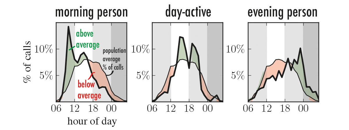
Daily Rhythms in Mobile Telephone Communication [PLoS One]
This is a very short post for those dabbling in the dark arts of network neuroscience. Everyone else, read this or this, they’re probably more fun anyway.
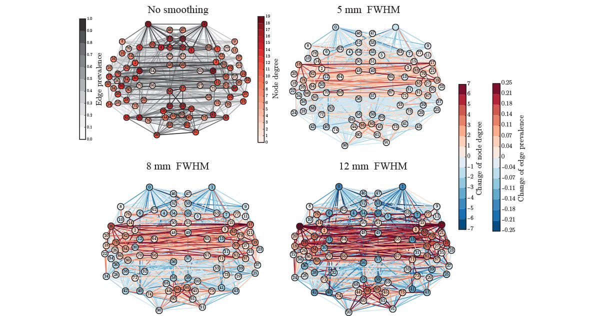
Q: When building ROI-level functional brain networks from fMRI data, should I apply spatial smoothing to the voxel time series?
A: No you should not, what were you thinking? See above; it messes up your degrees and links non-uniformly, and in general has weird effects. In any case, you already average your voxel time series to get your ROIs, which is brutal enough. For more, see our recent (open-access) paper in the European Journal of Neuroscience, with @TuomasAlakorkko and @eglerean and @hpsaarimaki and Onerva Korhonen.
Summary: Nodes in brain networks from fMRI are usually defined using ROI’s (Regions of Interest) so that each ROI node has a time series that is the average of the BOLD time series of the ROI’s voxels and links represent correlations between nodes. Here, we show that this averaging of voxel time series is problematic.
The human brain is a complex network of neurons. The problem is that there are about 10^12 of them with ~10^5 outgoing connections each; mapping out a network of this scale is not possible. Therefore, one needs to zoom out and look at the coarse-grained picture. This coarse-grained picture can be anatomical – a map of the large-scale wiring diagram between parts of the brain – or functional, indicating which parts of the brain tend to become active together under a given task.
But how should this coarse-graining be done in practice? How to define the nodes of a brain network –– what should brain nodes represent? In functional magnetic resonance imaging (fMRI), the highest level of detail is determined by the imaging technology. In a fMRI experiment, subjects are put inside a scanner that measures the dynamics of blood oxygenation in a 3D representation of the brain, divided into around 10,000 volume elements (voxels). Blood oxygenation is thought to correlate with the level of neural activity in the area. As each voxel contains about 5.5 million neurons, the network of voxels is significantly smaller than the network of neurons. However, it is still too large for many analysis tasks, and further coarse-graining is needed.
A typical way in the fMRI community is to group voxels into larger brain regions that are for historical reasons known as Regions of Interest (ROIs). This can be done in many ways, and there are many pre-defined maps (“brain atlases”) that define ROIs; these maps are based on anatomy, histology, or data-driven methods. It is common to use ROIs as the nodes of a brain functional network. The first step in constructing the brain network is to assign to each ROI a time series that is the average of the time series of its voxels measured in the imaging experiment. Then, to get the links, similarities between the ROI time series are calculated, usually with the Pearson correlation coefficient. The correlation between the two ROIs becomes their link weight. Often, only the strongest correlations are retained, and weak links are pruned from the network.
If the ROI approach is to work, the ROIs should be functionally homogeneous: their underlying voxels should behave approximately similarly. Otherwise, it is not clear what the brain network represents. Because this assumption hasn’t really been tested properly and because it is fundamentally important, we recently set out to explore whether it really holds.
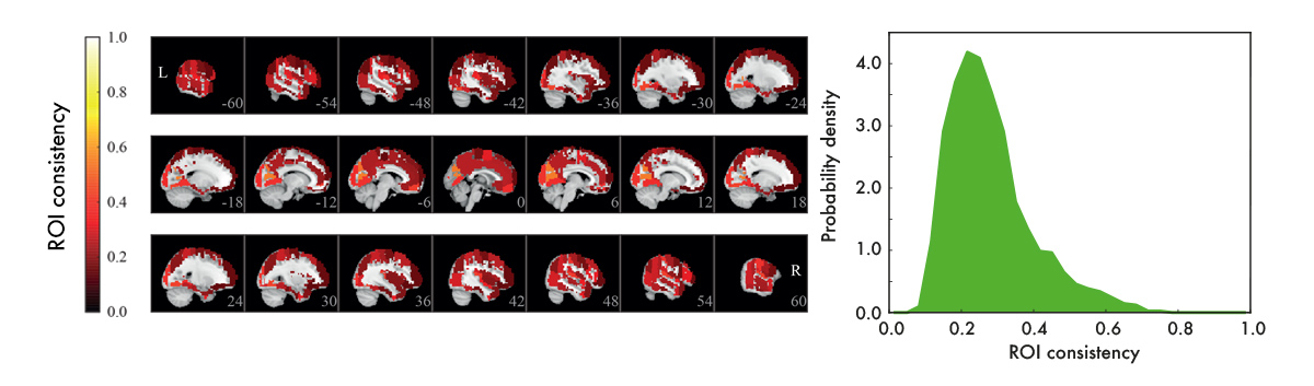
We used resting-state data – data recorded with subjects who are just resting in the scanner, instructed to do nothing – to construct functional ROI-level networks based on some available atlases. We defined a measure of ROI consistency that has a value of one if all the voxels that make up the ROI have identical time series (making the ROI functionally homogeneous, which is good), and a value of zero if the voxels do not correlate at all (making that ROI a bad idea, in general).
We found that consistency varied broadly between ROIs. While a few ROIs were quite consistent (values around 0.6), many were not (values around 0.2). There were many low-consistency ROIs in three commonly used brain atlases.
From the viewpoint of network analysis, the existence of many low-consistency ROIs is a bit alarming. We also observed strong links between low-consistency ROIs – how should this be interpreted? These links may be an artefact, as they disappear if we look at the voxel-level signals. This means that the source of the problem is probably the averaging of voxel signals into ROI time series. While this averaging can reduce noise, it can also remove the signal: at one extreme, if one subpopulation of voxels goes up while another goes down, the average signal is flat. More generally, if a ROI consists of many functionally different subareas, their average signal is not necessarily representative of anything.
In conclusion, we would recommend being careful with functional brain networks constructed using ROIs; at least, it would be good to go back to the voxel-level data to verify that the obtained results are indeed meaningful.
[PS: The definition of brain network nodes is not the only complicated issue in the study of functional brain networks. Even before one has to worry about node selection, a possible distortion has already taken place: preprocessing of the measurement data. We’ll continue this story soon.]
Ant colonies are complex systems par excellence. It’s almost as if the colony is the organism, not the ant. Ants follow simple behavioural patterns, depositing pheromones as they go and following trails of scent laid down by others. Because of their collective actions, the colony seems to have a life of its own, sprouting its foraging trails towards food sources much like a slime mold grows its branches along the shortest path to food. The colony appears to have its own reproductive cycle too: queens and males mate during the nuptial flight, and the impregnated queens then land to give birth to new colonies, like fertilized eggs. Ordinary workers play no role in reproduction; they are outside the germline.
But some species of ants behave in ways that are even more complex: they form supercolonies, networks of interconnected nests with hundreds of reproductive queens. In these supercolonies, queens and workers move freely between nests without eliciting aggression; they cooperate across nest boundaries. Ant supercolonies are the largest cooperative units known in nature: for some ants, they can extend for hundreds of kilometres. They are also among the strangest: their existence is difficult to explain from the point of view of gene-centric evolutionary theory. This has to do with altruism: relatedness among nestmates can be low, and workers will end up helping unrelated individuals that carry a different set of genes. It may even be that ant supercolonies represent an evolutionary dead end.
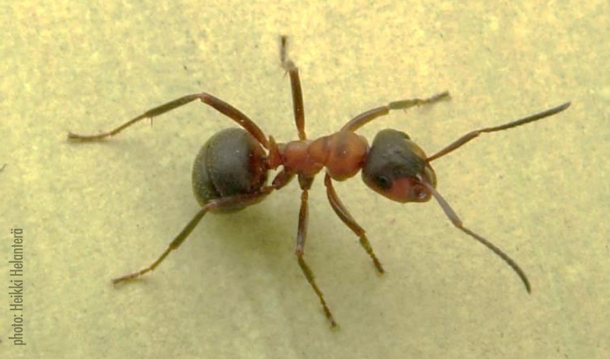
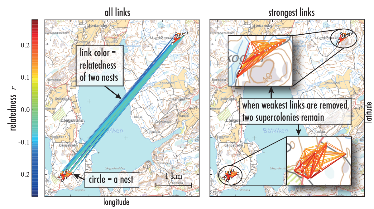
Recently, I had a chance to have some fun with the genetics of ant supercolonies. My colleagues Eva Schultner and Heikki Helanterä who work on ants had collected a number of samples from tens of nests of F. Aquilonia in southern Finland. As Eva and Heikki wanted to understand the genetic structure of F. Aquilonia supercolonies, the sampled ants were genotyped for estimating genetic similarities between the nests (for technical details, scroll down). From a network-science point of view, the nests and their similarities span a weighted spatial network: nests are nodes and pairwise genetic similarities are mapped to link weights. The resulting similarity network looks like this:
There are two supercolonies, one to the NE and one to the SW – the link weights inside the colonies are higher than between them, much like you would have for two communities in a social network. A closer look inside these two supercolonies (with methods more advanced than bare-bones network thresholding) revealed that there is a faint hint of substructure, of subclusters inside supercolonies. And because queens, workers, and pupae were genotyped separately and sampled at two time points, we could see that the genetic relationships between nests are not the same in terms of queens as they are in terms of workers, and not the same in spring as they are in summer when workers have started migrating.
This means that there may an extra layer of complexity in the genetics of ant supercolonies – fine structure in time and space, and in terms of class.
This work was published in Molecular Ecology last year. If you are interested in toying around with ant genetics, the data are available on Datadryad and my Python scripts can be found here: github.com/jsaramak/ants.
[Technical details: the ants were sequenced at 8 polymorphic microsatellite loci; microsatellites are nonsensical bits of DNA where a random sequence is repeated 5-50 times. They do not do anything and there is no selection pressure, and therefore microsatellite alleles are great for just seeing how close or far two populations are genetically. There are various measures for quantifying this: the simplest would be to see how often the same alleles appear in populations. In social-insect studies, the typical measure is the so-called relatedness (Queller & Goodnight 1989) and we used it in this work.]